Chapter 16 Model Selection for Prediction
\(\newcommand{\E}{\mathrm{E}}\) \(\newcommand{\Var}{\mathrm{Var}}\) \(\newcommand{\bmx}{\mathbf{x}}\) \(\newcommand{\bmH}{\mathbf{H}}\) \(\newcommand{\bmI}{\mathbf{I}}\) \(\newcommand{\bmX}{\mathbf{X}}\) \(\newcommand{\bmy}{\mathbf{y}}\) \(\newcommand{\bmY}{\mathbf{Y}}\) \(\newcommand{\bmbeta}{\boldsymbol{\beta}}\) \(\newcommand{\bmepsilon}{\boldsymbol{\epsilon}}\) \(\newcommand{\bmmu}{\boldsymbol{\mu}}\) \(\newcommand{\bmSigma}{\boldsymbol{\Sigma}}\) \(\newcommand{\XtX}{\bmX^\mT\bmX}\) \(\newcommand{\mT}{\mathsf{T}}\) \(\newcommand{\XtXinv}{(\bmX^\mT\bmX)^{-1}}\)
16.1 Variable Selection & Model Building
If we have a set of measured variables, a natural quesiton to ask is: Which variables do I include in the model? This is an important question, since our quantitative results and their qualitative interpretation all depend on what variables are in the model.
It can help to ask: Why not include every variable I have? There are several reasons why including every possible might not be optimal. These include:
- Scientific Interest – We may not be interested in relationships adjusted for all variables
- Interpretability – Having many (dozens, hundreds) of variables can make interpretation difficult.
- Multicollinearity – Adding many variables inflates the variances and standard errors.
- Overfitting – Too many variables, relative to the sample size, can result in a model that does not generalize well.
To get more specific in our approach to model selection, then we need to first determine what our modeling purpose is. In Prediction Modeling, our goal is to find model that best predicts outcome \(y\). In this case, we should choose a model based on minimizing prediction error and we don’t need to worry about \(p\)-values, \(se(\hat\bmbeta)\), or \(\beta\) interpretations. In Association Modeling, our goal is to estimate association between a chosen predictor(s) and the outcome and we should choose a model based on scientific knowledge.
The remainder of this chapter focuses on model selection for prediction; Section 17 covers how to choose variables for association modeling.
16.2 Prediction Error
When goal is prediction, we use prediction error to choose a model. For continuous variables, this is almost always quantified as Mean Squared Error: \[MSE(\hat{y}, y) = \E[(\hat y - y)^2]\] If the model is perfect, then \(\hat y_i = y_i\) and \(MSE(\hat y, y) = 0\). The further \(\hat y\) is from \(y\), the larger MSE will be.
For binary variables, we can use classification accuracy (see Section @ref()).
We calculate MSE by averaging over the data: \[\widehat{MSE}(\hat{y}, y) = \frac{1}{n}\sum_{i=1}^n (\hat{y}_i - y_i)^2\] It is critically important which data points arer used in \(\widehat{MSE}(\hat{y}, y)\). If we evaluate MSE using the same data used to fit the model, then we are using in-sample data. In-sample MSE will always be too optimistic, since we are using the data twice–once to estimate the \(\beta\)’s and once to calculate \(\widehat{MSE}\). In contrast, we can use a different set of data points, typically referred to as out-of-sample data, for calculating MSE. To get an accurate estimate of MSE, we always want to use out-of-sample data.
Instead of MSE, sometimes we use root mean squared error \(RMSE = \sqrt{MSE}\). RMSE is on the scale of the data (like standard deviation), which can make it easier to interpret. The model with smallest MSE is model with smallest RMSE, so either can be used for selection.
16.3 Model Selection & Evaluation Strategy
With a large dataset, the best approach is to split your data into three mutually exclusive sets:
- Training Data
- Validation Data
- Test Data
Once the data is split into these sets, the procedure for selecting a prediction model is:
- Training Data – Fit your candidate model(s) using the training data.
- Obtain estimates of the model coefficients (\(\beta\))
- Models can use different variables, transformations of \(x\), etc.
- Validation Data – Evaluate the performance of the models using training data observation.
- Estimates the out-of-sample error for predictions from each model
- Perform model selection: Choose the model with the best (lowest) MSE
- Test Data – Evaluate the performance of the chosen model using test data.
- Error estimated from validation data will be too low on average (because you chose the best model among many)
- Estimating error from an independent test dataset after you have chosen the model provides gold standard of model performance
- When do I have enough data to split into these three groups?
- Need good representation of predictor variables in all groups
- What is “large” enough depends on the particular setting
16.3.1 Synthetic Data Example
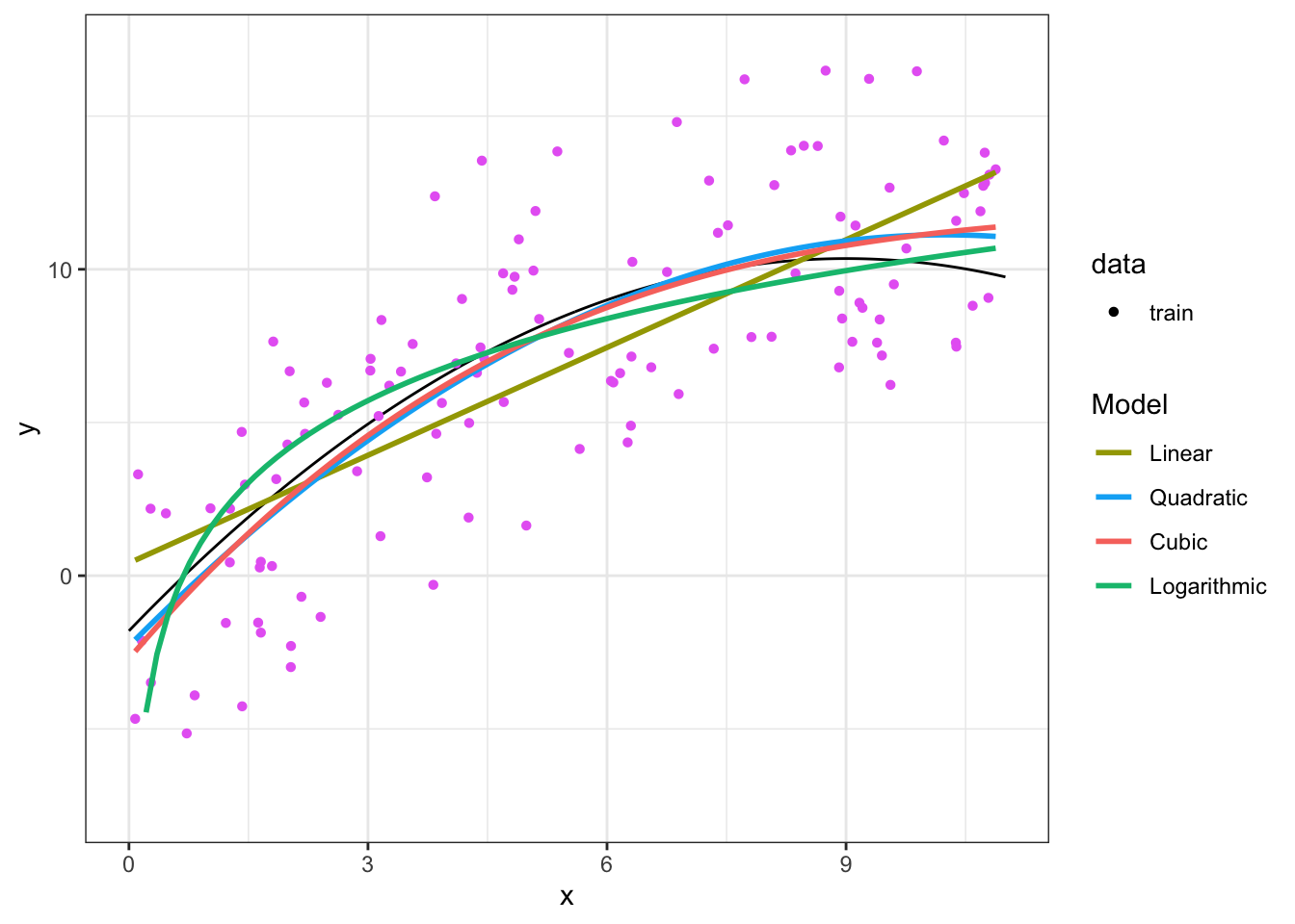
To see this in practice, let’s use a set of simulated data from the model \[Y_i = -1.8 + 2.7x_i - 0.15x_i^2 + \epsilon_i \qquad \epsilon_i\sim N(0, 3^2)\]
We have 200 data points, so let us split them up into three groups:
- 120 for training data
- 40 for validation data
- 40 for test data

16.3.2 Candidate Models
Let’s compare the following models for this data:
- \(\E[Y_i] = \beta_0 + \beta_1x_i\)
- \(\E[Y_i] = \beta_0 + \beta_1x_i +\beta_2x_i^2\)
- \(\E[Y_i] = \beta_0 + \beta_1x_i +\beta_2x_i^2 + \beta_3x_i^3\)
- \(\E[Y_i] = \beta_0 + \beta_1\log(x_i)\)
Steps for model selection:
- For each model: Fit model (i.e. compute \(\hat\bmbeta\)) in training data. Optional: Compute in-sample MSE in training data. (Skip this in practice, we’ll do this for illustration).
- For each model: Compute out-of-sample MSE in validation data
- Choose the model with lowest out-of-sample MSE as best
- Evaluate the out-of-sample MSE for the best model in test data
16.3.3 Linear Model Fit
Step 1: Fit the model to training data
## # A tibble: 2 × 5
##   term        estimate std.error statistic  p.value
##   <chr>          <dbl>     <dbl>     <dbl>    <dbl>
## 1 (Intercept)    0.413    0.599      0.690 4.91e- 1
## 2 x              1.17     0.0934    12.5   1.82e-23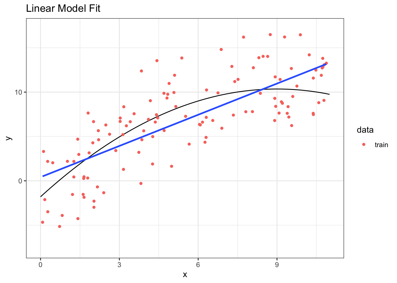
Step 1b: (Optional) Compute the in-sample MSE
\[\widehat{MSE}(\hat{y}, y) = \frac{1}{n}\sum_{i=1}^n (\hat{y}_i - y_i)^2\]
## [1] 11.16458Step 2: Compute the out-of-sample MSE in validation data
## [1] 13.5443916.3.4 Quadratic Model Fit
Step 1: Fit the model to training data
## # A tibble: 3 × 5
##   term        estimate std.error statistic  p.value
##   <chr>          <dbl>     <dbl>     <dbl>    <dbl>
## 1 (Intercept)     6.86     0.290     23.7  2.11e-46
## 2 poly(x, 2)1    42.3      3.18      13.3  3.47e-25
## 3 poly(x, 2)2   -12.6      3.18      -3.98 1.19e- 4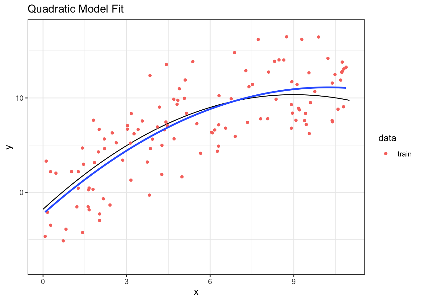
Step 1b: (Optional) Compute the in-sample MSE
## [1] 9.83214Step 2: Compute the out-of-sample MSE in validation data
## [1] 11.7297616.3.5 Cubic Model Fit
Step 1: Fit the model to training data.
## # A tibble: 4 × 5
##   term        estimate std.error statistic  p.value
##   <chr>          <dbl>     <dbl>     <dbl>    <dbl>
## 1 (Intercept)     6.86     0.291    23.6   4.55e-46
## 2 poly(x, 3)1    42.3      3.19     13.3   5.09e-25
## 3 poly(x, 3)2   -12.6      3.19     -3.97  1.25e- 4
## 4 poly(x, 3)3     1.65     3.19      0.518 6.05e- 1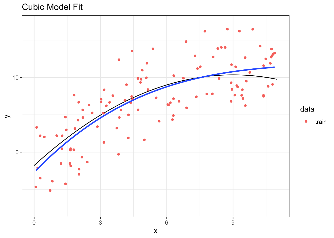
Step 1b: (Optional) Compute the in-sample MSE
## [1] 9.809451Step 2: Compute the out-of-sample MSE in validation data.
## [1] 11.9632716.3.6 Logarithmic Model Fit
Step 1: Fit the model to training data.
## # A tibble: 2 × 5
##   term        estimate std.error statistic  p.value
##   <chr>          <dbl>     <dbl>     <dbl>    <dbl>
## 1 (Intercept)     1.47     0.550      2.68 8.37e- 3
## 2 log(x)          3.86     0.323     12.0  4.43e-22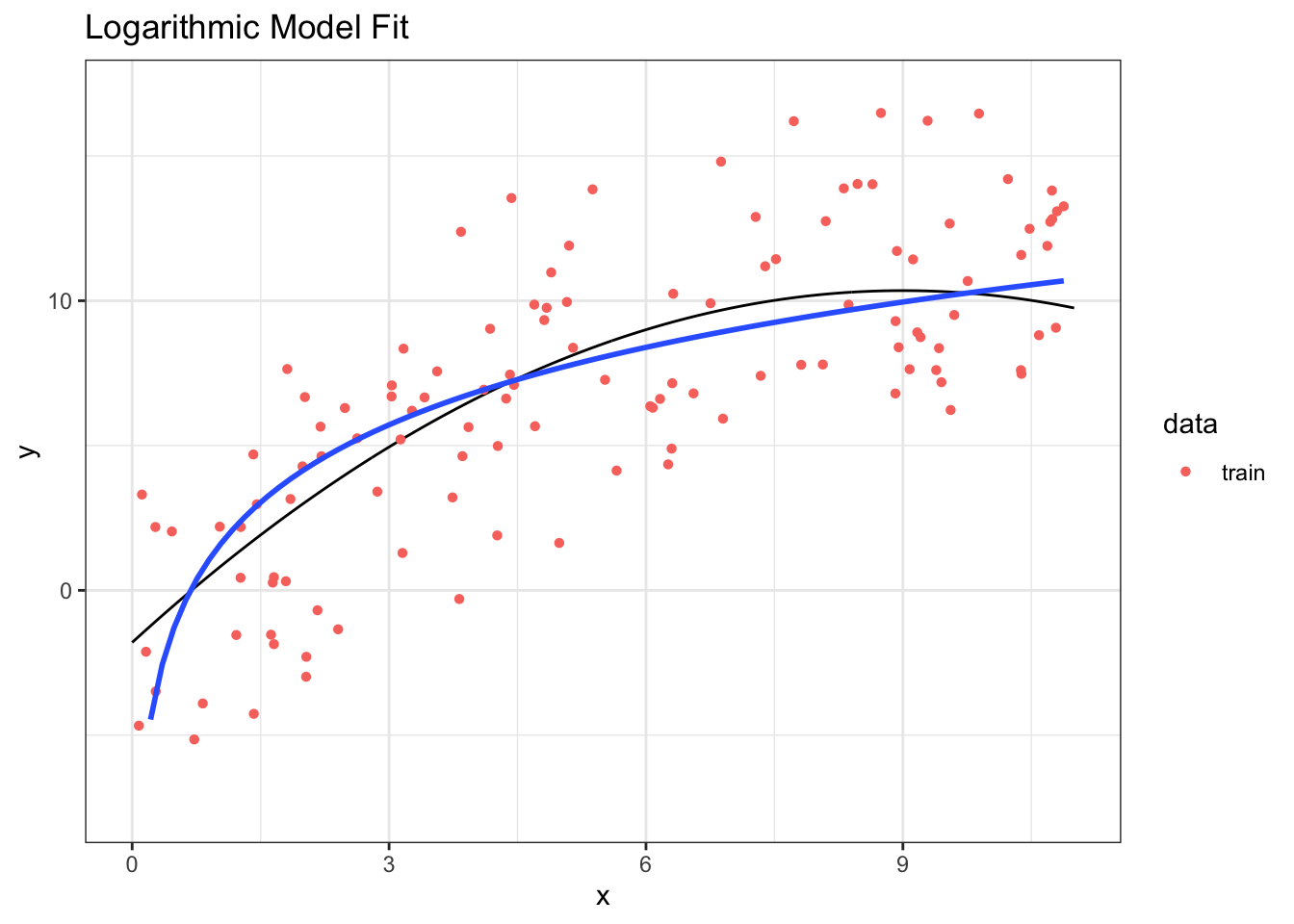
Step 1b: (Optional) Compute the in-sample MSE
## [1] 11.78063Step 2: Compute the out-of-sample MSE in validation data
## [1] 12.7850416.3.7 Comparing Model Fits
| # | Model for \(\E[Y]\) | In-sample MSE | Out-of-sample MSE |
|---|---|---|---|
| 1 | \(\beta_0 + \beta_1x_i\) | 11.16 | 13.54 |
| 2 | \(\beta_0 + \beta_1x_i +\beta_2x_i^2\) | 9.83 | 11.73 |
| 3 | \(\beta_0 + \beta_1x_i +\beta_2x_i^2 + \beta_3x_i^3\) | 9.81 | 11.96 |
| 4 | \(\beta_0 + \beta_1\log(x_i)\) | 11.78 | 12.78 |
Step 3: Choose model with smallest out-of-sample MSE
- Choose Model 2, which has smallest out-of-sample MSE
- Model 3 has smaller in-sample MSE, but larger out-of-sample MSE
- Example of overfitting to the data
16.3.9 Model Selection for Prediction Recap
- Training – Fit candidate models using the training data.
- Validation – Compute MSE of predictions for validation dataset; pick best model.
- Test – Evaluate the MSE of prediction from the chosen model using test data.
- You can fit many models in training stage, exploring data in many ways
- Only do validation and testing stages once; otherwise you will overfit
16.4 Cross-validation
16.4.1 Cross-validation
Main Idea: Use a single dataset to approximate having training, validation, and test data
- Create \(k\) CV groups/subsets from the full data
- \(k=10\) most often (= “10-fold” cross-validation)
- Repeat the following for each group:
- Creating “CV-training” data from all observations not in the current group and “CV-test” data from observations in the current group
- Fit the model(s) to the these “CV-training” data.
- Make predictions for the observations in the “CV-test” data
- Evaluate the prediction performance of each model, comparing CV predictions to observed values
- Approximates out-of-sample error since “CV-test” observations not used in model fitting.
- Choose the model with best prediction performance
Note: Estimate of accuracy for chosen model is still optimistic because of model selection. Best procedure would be to then evaluate on separate test data.
16.4.2 Example: Predicting Cereal Ratings
Let’s apply cross-validation to the cereals data, predicting ratings of each cereal.
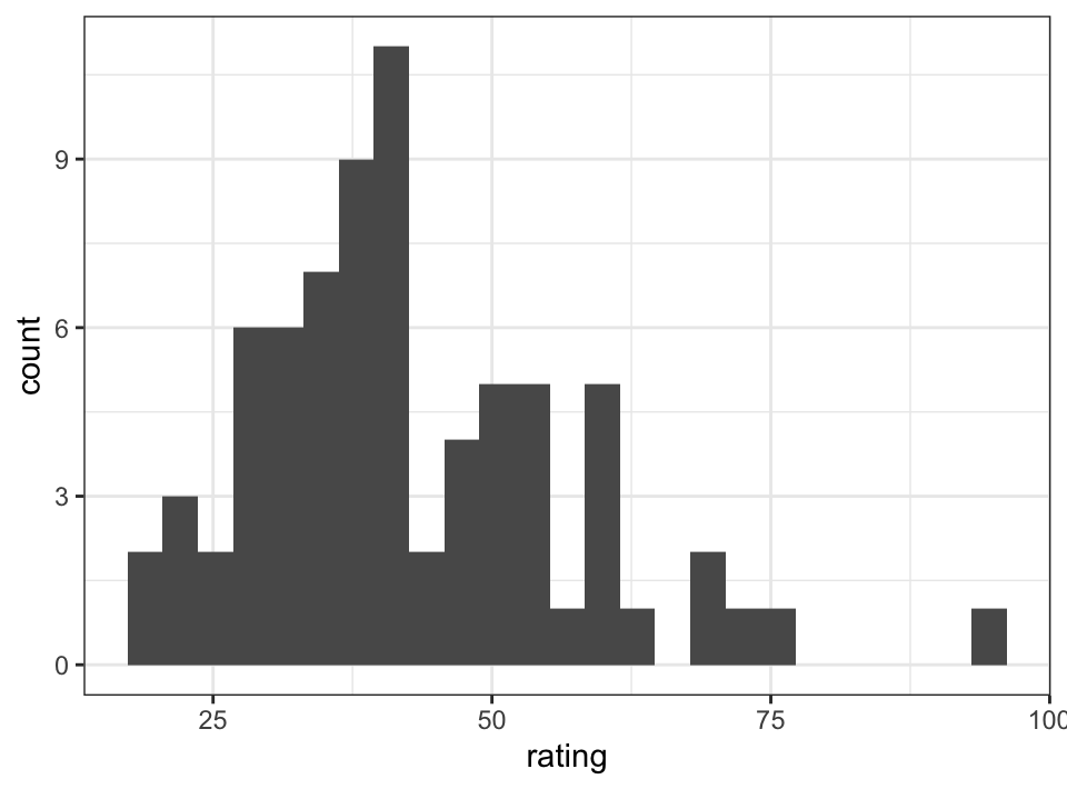
Let’s choose between 3 models:
Model 1: Manufacturer (Kellogg’s, General Mills, or other)
Model 2: Sugars, Vitamins, & Calories
Model 3: Manufacturer, Sugars, Vitamins, & Calories
Limiting to 3 models for simplicity. We could consider models with more variables, transformations, interactions, etc.
16.4.2.1 Creating CV Groups
- Create 10 CV groups from the full data
createFolds()fromcaretcan do this for you easily
set.seed(5)
k <- 10
flds <- createFolds(cereals$rating, k = k, list = TRUE,
                    returnTrain = FALSE)
str(flds)
## List of 10
## $ Fold01: int [1:7] 3 23 25 34 37 60 70
## $ Fold02: int [1:8] 10 15 32 51 56 62 68 72
## $ Fold03: int [1:7] 6 13 38 53 54 55 64
## $ Fold04: int [1:7] 11 20 22 31 41 44 50
## $ Fold05: int [1:8] 1 21 28 40 45 46 52 65
## $ Fold06: int [1:8] 7 9 18 30 33 42 43 69
## $ Fold07: int [1:8] 2 4 5 8 12 57 59 63
## $ Fold08: int [1:7] 14 24 26 48 61 67 73
## $ Fold09: int [1:7] 16 29 36 39 47 49 66
## $ Fold10: int [1:7] 17 19 27 35 58 71 7416.4.2.2 Fitting Model & Making Predictions
- For each CV group, fit model to training subset and make predictions for the test subset
## Create lists for storing predictions
## One element for each model
pred_list <- list(numeric(nrow(cereals)),
                  numeric(nrow(cereals)),
                  numeric(nrow(cereals)))
for (i in 1:k){
## Subset training data
train <- cereals[-flds[[i]],]
## Subset test data
test <- cereals[flds[[i]],]
## Fit each model
cereals_cvm1 <- lm(rating~mfr, data=train)
cereals_cvm2 <- lm(rating~sugars + vitamins + calories, data=train)
cereals_cvm3 <- lm(rating~mfr + sugars + vitamins + calories,
data=train)
## Store predictions
pred_list[[1]][flds[[i]]]=predict(cereals_cvm1,
newdata=test)
pred_list[[2]][flds[[i]]]=predict(cereals_cvm2,
newdata=test)
pred_list[[3]][flds[[i]]]=predict(cereals_cvm3,
newdata=test)
}16.4.3 CV using caret
The caret package can automate CV for us, which greatly simplifies this process. The primary function is train():
* Provide formula and data like normal.
* Set method="lm"
* Set trControl = trainControl(method = "cv")
## Linear Regression
##
## 74 samples
##  1 predictor
##
## No pre-processing
## Resampling: Cross-Validated (10 fold)
## Summary of sample sizes: 67, 67, 67, 68, 67, 66, ...
## Resampling results:
##
##   RMSE      Rsquared   MAE
##   12.71789  0.2815844  10.25323
##
## Tuning parameter 'intercept' was held constant at a value of TRUE
16.4.4 Cross-validation Summary
- Cross-validation is a way to approximate out-of-sample prediction when separate training/validation/test data are unavailable
- General Procedure:
- Split the data into groups
- For each group, make predictions using model fit to rest of data
- Compare models using \(y\) and cross-validation predictions \(\hat y\)
16.5 AIC & Information Criteria
What if we don’t have enough data to use a training/validation/test set or do cross-validation? We can use a different measure of model fit.
Information Criteria (IC) approaches are based on maximum likelihood (ML), which assumes a normal distribution for the data. The ML approach to estimation finds \(\beta\) and \(\sigma^2\) that maximize the log-likelihood \[\log L = -\frac{1}{2\sigma^2}(\bmy - \bmX\bmbeta)^\mT(\bmy - \bmX\bmbeta) - \frac{n}{2}\sigma^2 + constant\] Heuristically, we can think of the likelihood \(L\) as the probability of the data given a particular model. The value of the likelihood \(\log L\) can be used to measure how “good” the model fit is, where higher \(\log L\) would be better.
To use the likelihood for model selection, we need a penalty term to account for adding parameters. This is similar to the penalty term added in \(R_{Adj}^2\).
The most common information criteria for model selection are:
\(AIC\): \(-2 \log L + 2p\)
\(BIC\): \(-2 \log L + p \log(n)\)
\(AIC_C\): \(-2 \log L + 2p + \frac{2k(k+1)}{n - k - 1}\)
For each of these, a lower value indicates a better model.
One major advantage of these approaches is that they can be used to easily compare non-nested models. However, they don’t target prediction accuracy (i.e. MSE) directly, so in general they are not as useful for prediction model selection as the approaches described above. In particular, the training/validation/test and CV approaches can extend to non-statistical models, while the information criteria approaches require the existence of a likelihood.
16.6 Choosing Models to Compare
All of these approaches require set of candidate models to select from. If the number of variables is small, then we can use an “all subsets” approach in which we try every combination of variables we have. However, this quickly becomes computationally impractical as the number of variables grows. Instead, it can be helpful to use exploratory plots and descriptive statistics (evaluating these in the training data, not the full data) to select reasonable combinations of variables to consider.
16.7 Other Types of Models
Linear regression is not the only method for predicting a continuous variable. Other approaches in clude:
- LASSO/Ridge regression
- Neural Networks
- Random Forests
- Generalized additive models
Happily, the caret package supports all of these types of models and train() is specifically designed to help with fitting these kinds of models. More information is available at: